4. Data Preprocessing, Local Models and Tree-Based Models

4.1. Introduction

Machine Learning, as you now know, is based on statistical analysis of data. Data comes in many kinds of formats, resolutions, annotations, … and therefore should be processed before performing analysis. This is the first content of this practical. We will focus on regression tasks, as already defined in the previous practicals, showing to commonly used strategies. The practical is structured around five key objectives:

1. Understanding and applying essential data preprocessing techniques
   Before training a machine learning model, the data must be properly prepared. We will cover the following common preprocessing steps:

   • Handling missing values: strategies to impute or remove data with missing entries.

   • Feature scaling and normalization: ensuring features are on comparable scales to improve model performance.

   • Encoding categorical variables: transforming non-numeric data (e.g., categories) into numerical representations suitable for machine learning algorithms.

2. Implementing the K-Nearest Neighbors (KNN) algorithm from scratch
   We will write a simple, “vanilla” version of the KNN algorithm for regression tasks. This implementation will help demystify how KNN works by reinforcing the idea of prediction based on similarity in feature space.

3. Training and evaluating tree-based regression models
   We will work with two popular types of decision-tree-based models for regression:

   • Regression trees: models that recursively split the data space into regions to predict a continuous output.

   • Random Forests: an ensemble method that combines multiple decision trees to improve predictive accuracy and reduce overfitting.

4. Interpreting feature importances in tree-based models
   One advantage of tree-based models is their ability to estimate the relative importance of each input feature. We will learn how to extract and interpret these feature importances to gain insights into which variables are most influential in the prediction.

5. Using scikit-learn Pipelines to streamline preprocessing and modeling
   To ensure clean and reproducible workflows, we will introduce scikit-learn pipelines, which allow us to:

   • Chain together preprocessing steps and model training into a single object.

   • Simplify cross-validation and hyperparameter tuning.

   • Prevent data leakage by ensuring that preprocessing is properly applied to both training and test data.

By the end of this practical, you should be able to preprocess real-world data appropriately, implement a basic regression model, use tree-based models effectively, and combine preprocessing and modeling steps into a coherent, automated pipeline using scikit-learn.

4.1.1. Important precision about the evaluation metric used in this practical

In this practical, we will use the Mean Squared Error (MSE) as a convenient shorthand for the estimated Mean Integrated Squared Error \((\widehat{\mathrm{MISE}})\). Indeed, in practice, we rarely know the true MISE and instead rely on estimates obtained via techniques like \(K\)-fold cross-validation or leave-one-out (LOO) cross-validation. So keep in mind that when we refer to the MSE in these contexts, what we are really computing is an estimation of \(\widehat{\mathrm{MISE}}\) from our data.

4.1.2. Data preprocessing overview

Data preprocessing is the foundation of any successful machine learning project. Many Machine Learning models see their performances degraded when trained on poorly preprocessed data. Key steps include:

• Handling Missing Values: Missing data can bias results if not addressed. This problem affects many models—such as linear models, support vector machines (SVMs), and neural networks—but it is particularly critical for distance-based algorithms like KNN where missing feature values can disrupt the calculation of distances, leading to inaccurate outcomes. Common strategies for handling missing values include:

  • Dropping rows/columns with missing data.

  • Imputing missing data using simple statistics (mean, median) or more sophisticated methods like KNNImputer.
    
    

• Normalization / Scaling: Many algorithms assume features are on similar scales. Without proper scaling, features with larger numerical ranges may dominate those with smaller ranges, potentially biasing the model’s results. Common scaling strategies include:

  • Standardization: Transform features to have zero mean and unit variance.

  • Min-Max Scaling: Scale features to a fixed \([0,1]\) range.
    
    

• Dealing with Categorical Variables: Categorical variables must be converted to a numeric representation that preserves meaningful differences. Common strategies for dealing with categorical variables include:

  • Label Encoding: Assign an integer to each category (useful if there is an ordinal relationship).

  • One-Hot Encoding (Dummy Encoding): Create a new binary column for each category (common for nominal features). This approach can cause a significant increase in input dimensionality (see the curse of dimensionality).

4.2. K-Nearest Neighbors

💡Did you know ? The \(K\)-Neighrest Neighbors algorithm was first proposed in Fix and Hodges [FH51].

The \(K\)-Nearest Neighbors (KNN) algorithm is a local modeling approach that infers its prediction from the data points closest (in some metric) to a query. Suppose we have a training set of inputs \(\{x_i\}\) with associated labels or targets \(\{y_i\}\). For a new query point \(q\):

1. Distance computation: Compute the distance (e.g., Euclidean) between \(q\) and each training example \(x_i\).

2. Ranking: Sort or rank the training points by increasing distance to \(q\).

3. Neighborhood selection: Identify the subset of the \(K\) nearest neighbors \(\{x_{[1]}, \dots, x_{[K]}\}\) where \(y_{[i]}\) denotes the label of neighbor \(x_{[i]}\).

4. Regression or classification: KNN can be viewed as a local estimator of the conditional expectation \(\mathbb{E}[y|x=q]\).

For regression tasks, the simplest approach is to average the targets of the \(K\) nearest neighbors:

\[ \hat{y}(q) = \frac{1}{K}\sum_{i=1}^{K} y_{[i]}. \]

Alternatively, a local linear model may be used:

\[ \hat{y}(q) = \hat{a}^T q + \hat{b}, \]

where \(\hat{a}\) and \(\hat{b}\) are estimated (locally) by least-squares on the neighbors.

For classification, one can estimate the conditional probability of belonging to a specific class (e.g., class “1”) by the proportion of neighbors labeled “1”:

\[ \hat{p}_1(q) = \frac{1}{K}\sum_{i=1}^{K} y_{[i]}. \]

A threshold (e.g., 0.5) can then be used to decide the class label.

The key hyperparameter here is \(K\). A smaller \(K\) reduces bias but increases variance, while a larger \(K\) produces a smoother model at the risk of higher bias. KNN’s performance also heavily depends on the distance metric, especially when features have different scales or include categorical variables (which may require specialized encodings or distance definitions).

4.3. Regression Trees

Regression trees rely on a tree-based structure of internal nodes (where decisions are made) and terminal nodes (leaves), which partition the input space into mutually exclusive regions, each associated with a simple (often constant) local model. Its construction begins with a tree growing phase: starting from the root node that contains all data, we recursively choose a split that best reduces the empirical error. Specifically, for a node \(t\) containing \(N(t)\) samples, we define

\[ R_{\mathrm{emp}}(t) \;=\; \min_{\alpha_t} \sum_{i=1}^{N(t)} L\bigl(y_i,\;h_t(x_i,\;\alpha_t)\bigr), \]

where \(L\) is typically the squared error \((y - \hat{y})^2\) for regression. Given a potential split \(s\) dividing \(t\) into children \(t_l\) and \(t_r\), we consider the decrease in empirical error:

\[ \Delta E(s,\;t) \;=\; R_{\mathrm{emp}}(t)\;-\;\bigl(R_{\mathrm{emp}}(t_l)\;+\;R_{\mathrm{emp}}(t_r)\bigr). \]

We choose the split \(s^*\) maximizing \(\Delta E\), partition the dataset accordingly, and repeat the procedure recursively until no further improvement is found or a stopping criterion is met. This exhaustive splitting often yields a very large tree that overfits the data.

To address overfitting, a cost-complexity pruning procedure is commonly used. Introducing a complexity parameter \(\lambda \ge 0\) that penalizes the number of leaf nodes, we define the cost-complexity measure:

\[ R_{\lambda}(T) = R_{\mathrm{emp}}(T) + \lambda \, |T|, \]

where \(|T|\) is the number of terminal nodes (leaves) in tree \(T\).

• By gradually increasing \(\lambda\), we obtain a sequence of subtrees:

\[ T_{\max} \supset T_{L-1} \supset \dots \supset T_2 \supset T_1. \]

Each has fewer leaves. We consider all admissible subtrees \(T_t \subset T\) of the large tree and compute the smallest

\[ \lambda_t = \frac{R_{\mathrm{emp}}(T) - R_{\mathrm{emp}}(T_t)}{|T| - |T_t|} \]

that yields a lower cost. We select the subtree that minimizes \(R_{\lambda}(T)\) (the best balances between empirical error and model complexity). The final tree structure is typically chosen via cross-validation or held-out validation to find the best \(\lambda\). A more visual representation of tree-based models, an animated version of decision trees (classification) can be found here.

Random Forest have been first presented in Ho [Ho98].

4.4. Random Forests

A Random Forest (RF), is an ensemble learning technique designed to reduce the variance of decision trees by combining two main ideas:

1. Bootstrap Sampling (Bagging): We generate \(B\) bootstrap datasets, each by sampling (with replacement) from the original training data.

2. Random Feature Selection (Feature Bagging): At each split, a random subset of \(n' < n\) features is chosen, and the best split is found only among those \(n'\) features.

Hence, each tree \(h_b(\mathbf{x}, \alpha_b)\) is built from a different resampled dataset and uses only a random subset of features at each split. As a result, the trees are more decorrelated and often are not pruned heavily.

Formally, for a regression task:

\[ h_{\mathrm{rf}}(\mathbf{x}) = \frac{1}{B} \sum_{b=1}^{B} h_b(\mathbf{x}, \alpha_b), \]

i.e., the average of all tree predictions. (In classification, we take the majority vote.)

4.4.1. Why does this reduce variance?

Suppose each tree \(h_b\) has variance \(\sigma^2\) and they have pairwise correlation \(\rho\). The variance of the RF predictor \(h_{\mathrm{rf}}\) can be approximated as:

\[ \mathrm{Var}[h_{\mathrm{rf}}] \approx \frac{(1 - \rho)\,\sigma^2}{B} + \rho\,\sigma^2, \]

which shows that increasing \(B\) (the number of trees) reduces the first term, while lowering the correlation \(\rho\) among trees reduces overall variance. Random feature selection helps reduce \(\rho\), because each tree sees a different subset of features.

4.4.2. Main Hyperparameters

1. \(B\): the number of trees in the forest.

2. \(n'\): the number of randomly selected features at each split (often \(\sqrt{n}\) by default in classification).

3. Tree parameters: e.g., maximum depth, minimum samples per leaf, etc.

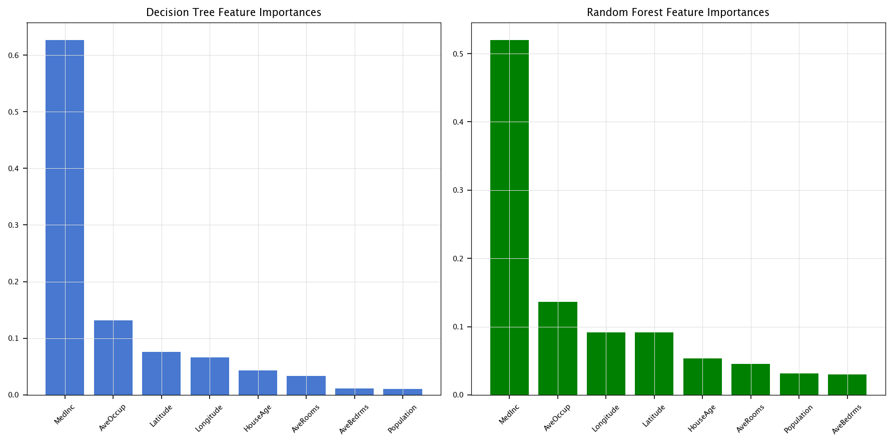
In practice, random forests typically provide strong performance out of the box and are less sensitive to hyperparameter tuning compared to single trees or more complex models. They also allow computing a useful estimate of feature importance by measuring, for each variable, how much it contributes to the cost function improvement across all splits in all trees.

4.5. Feature Importances

Most scikit-learn models allows you to estimate how each feature contribues to the final prediction. For example, for tree-based models, both DecisionTreeRegressor and RandomForestRegressor in scikit-learn store a feature_importances_ attribute after fitting. This gives an estimate of how much each feature contributed to reducing the split criterion (e.g., MSE).

4.6. Scikit-learn Pipelines

Pipelines in scikit-learn let us combine data preprocessing (e.g., imputation, scaling) and model training (e.g., a random forest) into a single workflow object. Below is a simple example:

from sklearn.pipeline import Pipeline
from sklearn.preprocessing import StandardScaler
from sklearn.linear_model import LinearRegression
from sklearn.impute import SimpleImputer

example_pipeline = Pipeline([
    ("imputer", SimpleImputer(strategy="mean")),
    ("scaler", StandardScaler()),
    ("regressor", LinearRegression())
])

from sklearn.base import BaseEstimator, TransformerMixin
from sklearn.ensemble import RandomForestRegressor

class AddConstantTransformer(BaseEstimator, TransformerMixin):
    """
    Custom transformer that adds a constant value to all features.
    """
    def __init__(self, constant=0.0):
        self.constant = constant

    def fit(self, X, y=None):
        return self

    def transform(self, X, y=None):
        return X + self.constant

custom_pipeline = Pipeline([
    ("imputer", SimpleImputer(strategy="mean")),
    ("custom_add_constant", AddConstantTransformer(constant=1.0)),
    ("scaler", StandardScaler()),
    ("regressor", RandomForestRegressor(n_estimators=10, random_state=42))
])

4.7. Exercises

4.7.1. California Housing

1. Load the well-known California Housing regression dataset using the following function:

from sklearn.datasets import fetch_california_housing

2. Explore the dataset (distribution, summary statistics).

3. Check for missing values. If the dataset does not contain missing values, artificially introduce some for the purpose of this exercice. Then, handle missing values by:

   • Dropping them (simple approach).

   • Imputing them (mean or median).

   • Using a more sophisticated method (e.g., KNNImputer).

4. Normalize the features (using e.g., StandardScaler). Remember that, as all processing steps, scaling is fit on the training set (not on the entire dataset) to avoid biasing the test set!

5. Preserve original vs. processed versions of the data for comparison.

4.7.2. Solution

4.7.2.1. Dataset and exploration

For this exercise, we will use the California Housing dataset from sklearn.datasets.fetch_california_housing. It contains features related to California housing data, and the target is the average house value.

Alternatively, if you would like test your solution on other datasets, scikit-learn provides other built-in datasets, such as:

• Diabetes (a small dataset with 10 features for a regression task on disease progression).

• Linnerud (exercise/physiological data, a small multi-output regression problem). If you want a dataset with even more features or complexity, you could consider Ames Housing or Kaggle House Price, both of which have many categorical and numeric features but may require additional steps to download or preprocess. You can also explore the UCI Machine Learning Repository for a wide range of tabular datasets.

import numpy as np
import pandas as pd
from sklearn.datasets import fetch_california_housing

cal_housing = fetch_california_housing()
X_original = pd.DataFrame(cal_housing.data, columns=cal_housing.feature_names)
y_original = pd.Series(cal_housing.target, name='Target')

print("Shape of the feature matrix:", X_original.shape)
print("Shape of the target vector:", y_original.shape)

X_original.info()
display(X_original.describe())

Shape of the feature matrix: (20640, 8)
Shape of the target vector: (20640,)
<class 'pandas.core.frame.DataFrame'>
RangeIndex: 20640 entries, 0 to 20639
Data columns (total 8 columns):
 #   Column      Non-Null Count  Dtype  
---  ------      --------------  -----  
 0   MedInc      20640 non-null  float64
 1   HouseAge    20640 non-null  float64
 2   AveRooms    20640 non-null  float64
 3   AveBedrms   20640 non-null  float64
 4   Population  20640 non-null  float64
 5   AveOccup    20640 non-null  float64
 6   Latitude    20640 non-null  float64
 7   Longitude   20640 non-null  float64
dtypes: float64(8)
memory usage: 1.3 MB

	MedInc	HouseAge	AveRooms	AveBedrms	Population	AveOccup	Latitude	Longitude
count	20640.000000	20640.000000	20640.000000	20640.000000	20640.000000	20640.000000	20640.000000	20640.000000
mean	3.870671	28.639486	5.429000	1.096675	1425.476744	3.070655	35.631861	-119.569704
std	1.899822	12.585558	2.474173	0.473911	1132.462122	10.386050	2.135952	2.003532
min	0.499900	1.000000	0.846154	0.333333	3.000000	0.692308	32.540000	-124.350000
25%	2.563400	18.000000	4.440716	1.006079	787.000000	2.429741	33.930000	-121.800000
50%	3.534800	29.000000	5.229129	1.048780	1166.000000	2.818116	34.260000	-118.490000
75%	4.743250	37.000000	6.052381	1.099526	1725.000000	3.282261	37.710000	-118.010000
max	15.000100	52.000000	141.909091	34.066667	35682.000000	1243.333333	41.950000	-114.310000

4.7.2.2. Handling Missing Values

Although the California Housing dataset typically does not contain missing values, let’s artificially introduce some missing values for demonstration. We will then show three approaches:

1. Dropping rows with missing values.

2. Imputing with mean or median.

3. KNNImputer or another advanced method.

An advanced method: KNNImputer

KNNImputer uses a K-Nearest Neighbors approach to fill missing entries: for each row that has missing features, it finds the nearest k rows (in feature space) that do not have missing values in those columns, and uses their values (e.g., average) to impute the missing ones. This can often be more accurate than a simple mean or median if the data has local structure—rows that are similar in some features are likely also similar in the others.

from sklearn.model_selection import train_test_split
from sklearn.impute import KNNImputer

missing_mask = np.random.rand(*X_original.shape) < 0.01
X_missing = X_original.copy()
X_missing[missing_mask] = np.nan

print("--- Number of missing values (artificial) ---")
print(X_missing.isnull().sum())

X_train_full, X_test_full, y_train_full, y_test_full = train_test_split(
    X_missing, y_original, test_size=0.2, random_state=42
)

X_train_drop = X_train_full.dropna(axis=0)
y_train_drop = y_train_full.loc[X_train_drop.index]
X_test_drop = X_test_full.dropna(axis=0)
y_test_drop = y_test_full.loc[X_test_drop.index]

print("--- After Dropping Missing Values ---")
print("Training set size:", X_train_drop.shape)
print("Test set size:", X_test_drop.shape)

from sklearn.impute import SimpleImputer

mean_imputer = SimpleImputer(strategy='mean')
X_train_mean = mean_imputer.fit_transform(X_train_full)
X_test_mean = mean_imputer.transform(X_test_full)

median_imputer = SimpleImputer(strategy='median')
X_train_median = median_imputer.fit_transform(X_train_full)
X_test_median = median_imputer.transform(X_test_full)

knn_imputer = KNNImputer(n_neighbors=3)
X_train_knn = knn_imputer.fit_transform(X_train_full)
X_test_knn = knn_imputer.transform(X_test_full)

--- Number of missing values (artificial) ---
MedInc        195
HouseAge      201
AveRooms      205
AveBedrms     219
Population    191
AveOccup      206
Latitude      177
Longitude     223
dtype: int64
--- After Dropping Missing Values ---
Training set size: (15284, 8)
Test set size: (3798, 8)

4.7.2.3. Dealing with Categorical Values

In this dataset, we have only numerical features. However, real-world datasets often include categorical variables. Two popular encoding strategies are:

1. Label Encoding: Each category is assigned an integer.

2. One-Hot Encoding (Dummy Encoding): Create a new binary column for each category.

Below is a small example using a synthetic dataframe containing a categorical column.

from sklearn.preprocessing import LabelEncoder

example_df = pd.DataFrame({
    "Size": ["Small", "Medium", "Large", "Medium", "Small"],
    "Weight": [1.0, 2.3, 5.5, 2.0, 1.1]
})

label_encoder = LabelEncoder()
example_df["Size_label"] = label_encoder.fit_transform(example_df["Size"])

one_hot_df = pd.get_dummies(example_df, columns=["Size"], prefix="Size")

Original DataFrame with Label Encoding:

display(example_df)

	Size	Weight	Size_label
0	Small	1.0	2
1	Medium	2.3	1
2	Large	5.5	0
3	Medium	2.0	1
4	Small	1.1	2

DataFrame with One-Hot Encoding:

display(one_hot_df)

	Weight	Size_label	Size_Large	Size_Medium	Size_Small
0	1.0	2	False	False	True
1	2.3	1	False	True	False
2	5.5	0	True	False	False
3	2.0	1	False	True	False
4	1.1	2	False	False	True

We’ll stick to numeric data for the main practical, but this is how you’d handle categorical features.

4.7.2.4. Normalization/Scaling

Scaling is critical for distance-based methods. We will use StandardScaler, which transforms each feature to have zero mean and unit variance, but note that MinMaxScaler is also a standard.

Remember: Always fit the scaler on the training set, then apply the same transformation to the test set. This prevents data leakage and preserves the integrity of the test data.

from sklearn.preprocessing import StandardScaler

scaler = StandardScaler()
X_train_scaled = scaler.fit_transform(X_train_mean)
X_test_scaled = scaler.transform(X_test_mean)

X_train_final = X_train_scaled
X_test_final = X_test_scaled
y_train_final = y_train_full
y_test_final = y_test_full

4.7.3. Vanilla KNN Implementation

1. Split your data into training and test sets (we should have already done that in the previous exercise).

2. Implement a vanilla KNN regressor from scratch (no scikit-learn for this part).

3. Choose a value of \(k\) (e.g., 3, 5, 7).

4. Compare predictions with the true values using Mean Squared Error (MSE).

4.7.3.1. Solution

On this graph, we clearly see that there is an optimal value for the number of neighbors to use: a value too small increases the variance of the predictions while a value too high increases the bias. The optimal value, of course, depends on the problem definition and on the training data.

import matplotlib.pyplot as plt
plt.style.use(['seaborn-v0_8-muted', 'practicals.mplstyle'])
from sklearn.metrics import mean_squared_error
from tqdm.auto import tqdm

def euclidean_distance(x1, x2):
    return np.sqrt(np.sum((x1 - x2) ** 2))

def knn_regressor(X_train, y_train, X_test, k=3):
    """
    A simple KNN regressor (manual implementation).
    - X_train: training features (numpy array)
    - y_train: training targets (numpy array)
    - X_test: test features (numpy array)
    - k: number of neighbors to consider
    """
    predictions = []
    for test_point in tqdm(X_test):
        distances = [euclidean_distance(test_point, x_train) for x_train in X_train]
        k_indices = np.argsort(distances)[:k]
        prediction = np.mean(y_train[k_indices])
        predictions.append(prediction)
    return np.array(predictions)

from scipy.spatial import distance

def knn_regressor_fast(X_train, y_train, X_test, k=3):
    """
    A faster KNN regressor using vectorized distance computation.
    """
    dists = distance.cdist(X_test, X_train, metric='euclidean')
    k_indices = np.argpartition(dists, kth=k, axis=1)[:, :k]
    predictions = np.mean(y_train[k_indices], axis=1)
    return predictions

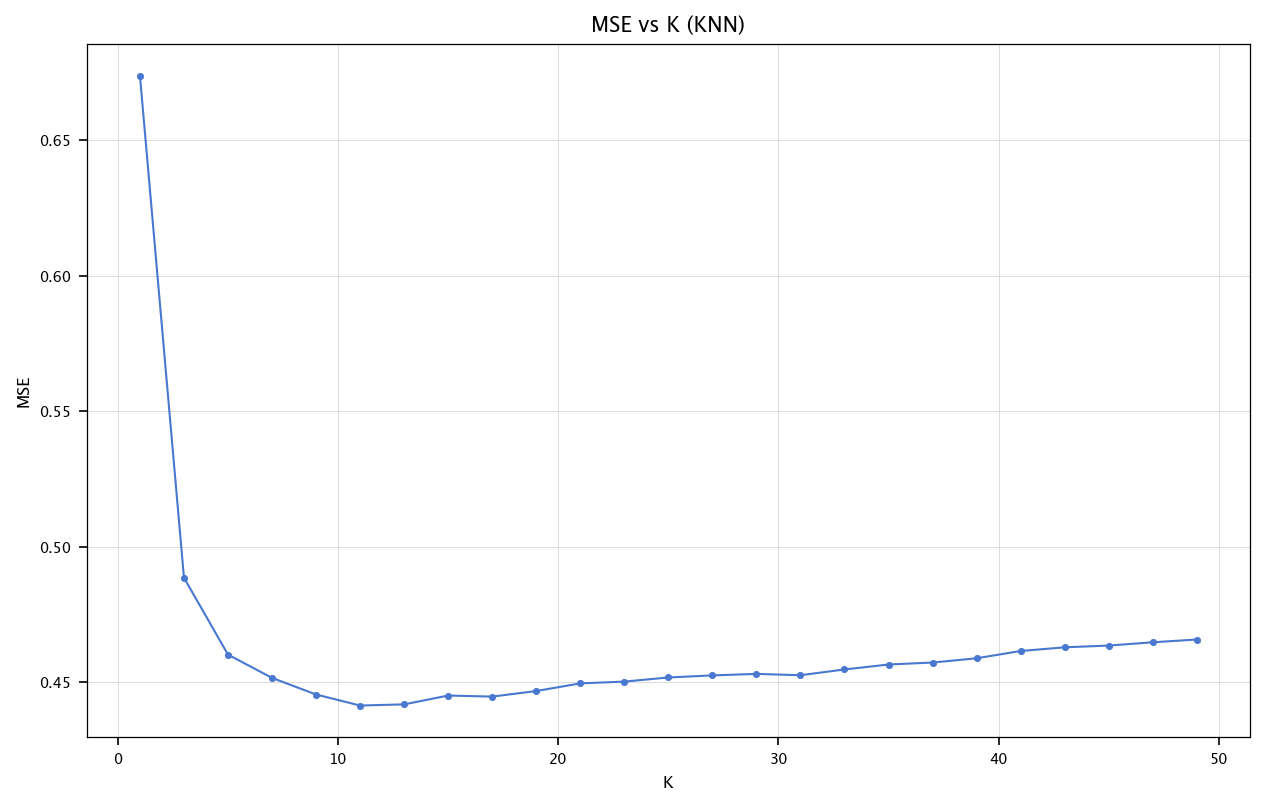
mses_knn = []
for k in tqdm(range(1, 51, 2)):
  y_pred_knn = knn_regressor_fast(X_train_final, y_train_final.values, X_test_final, k=k)
  mses_knn.append(mean_squared_error(y_test_final, y_pred_knn))

plt.figure(figsize=(10, 6))
plt.plot(list(range(1, 51, 2)), mses_knn, marker='o')
plt.title("MSE vs K (KNN)")
plt.xlabel("K")
plt.ylabel("MSE")
plt.grid("on")
plt.show()

4.7.4. Regression Trees and Random Forests

1. Train a regression tree on the training set.

2. Train a random forest on the training set.

3. Evaluate both models using MSE.

4. Compare their performance with your KNN model.

5. Determine how modifying the max_depth (for the regression trees) and n_estimators (for the random forests) impacts the performances of the model. Plot these results graphically.

6. Plot the features importance of the best model with the optimal parameters

4.7.5. Solution

4.7.5.1. Implementation with scikit-learn

from sklearn.tree import DecisionTreeRegressor
from sklearn.ensemble import RandomForestRegressor

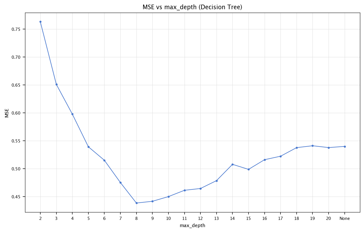
tree_reg = DecisionTreeRegressor(max_depth=9, random_state=42)
tree_reg.fit(X_train_final, y_train_final)
y_pred_tree = tree_reg.predict(X_test_final)
mse_tree = mean_squared_error(y_test_final, y_pred_tree)

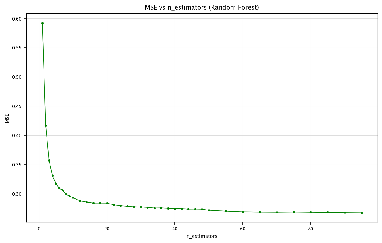
forest_reg = RandomForestRegressor(n_estimators=60, random_state=42)
forest_reg.fit(X_train_final, y_train_final)
y_pred_forest = forest_reg.predict(X_test_final)
mse_forest = mean_squared_error(y_test_final, y_pred_forest)

print("Comparison of MSE:")
print(f"KNN (k=13): {mean_squared_error(y_test_final, knn_regressor_fast(X_train_final, y_train_final.values, X_test_final, k=13)):.4f}")
print(f"Decision Tree: {mse_tree:.4f}")
print(f"Random Forest: {mse_forest:.4f}")

Comparison of MSE:

KNN (k=13): 0.4419
Decision Tree: 0.4417
Random Forest: 0.2693

Exploring Key Parameters

Decision Tree: max_depth

We can examine how max_depth (the maximum number of splits from the root to the leaf) affects performance.

depths = list(range(2, 21)) + [None]
mse_values_tree = []

for d in depths:
    dt = DecisionTreeRegressor(max_depth=d, random_state=42)
    dt.fit(X_train_final, y_train_final)
    y_pred_dt = dt.predict(X_test_final)
    mse_values_tree.append(mean_squared_error(y_test_final, y_pred_dt))

plt.figure(figsize=(10, 6))
plt.plot([str(d) for d in depths], mse_values_tree, marker='o')
plt.title("MSE vs max_depth (Decision Tree)")
plt.xlabel("max_depth")
plt.ylabel("MSE")
plt.grid("on")
plt.show()

Random Forest: n_estimators

Similarly, we can see how n_estimators (the number of trees in the forest) impacts the MSE.

estimators_range = list(range(1, 10))+list(range(10, 50, 2))+list(range(50, 100, 5))
mse_values_rf = []

for n in tqdm(estimators_range):
    rf = RandomForestRegressor(n_estimators=n, random_state=42)
    rf.fit(X_train_final, y_train_final)
    y_pred_rf = rf.predict(X_test_final)
    mse_values_rf.append(mean_squared_error(y_test_final, y_pred_rf))

plt.figure(figsize=(10, 6))
plt.plot(estimators_range, mse_values_rf, marker='o', color='green')
plt.title("MSE vs n_estimators (Random Forest)")
plt.xlabel("n_estimators")
plt.ylabel("MSE")
plt.grid("on")
plt.show()

4.7.5.2. Feature importance with the best models

Based on the experiments above, let’s define user-chosen parameters for the best (or at least improved) Decision Tree and Random Forest, then compute and display their feature importances.

Feel free to update max_depth and n_estimators according to the results you obtained above. Later, we will see how this can be used as a feature selection method.

max_depth = 9
n_estimators = 60 

best_tree = DecisionTreeRegressor(max_depth=max_depth, random_state=42)
best_tree.fit(X_train_final, y_train_final)

best_forest = RandomForestRegressor(n_estimators=n_estimators, random_state=42)
best_forest.fit(X_train_final, y_train_final)

feature_names = X_original.columns

tree_importances = best_tree.feature_importances_
forest_importances = best_forest.feature_importances_

tree_sorted_idx = np.argsort(tree_importances)[::-1]
forest_sorted_idx = np.argsort(forest_importances)[::-1]

plt.figure(figsize=(12, 6))
plt.subplot(1, 2, 1)
plt.title("Decision Tree Feature Importances")
plt.bar(range(len(tree_importances)), tree_importances[tree_sorted_idx], align='center')
plt.xticks(range(len(tree_importances)), feature_names[tree_sorted_idx], rotation=45)
plt.grid("on")
plt.subplot(1, 2, 2)
plt.title("Random Forest Feature Importances")
plt.bar(range(len(forest_importances)), forest_importances[forest_sorted_idx], align='center', color='green')
plt.xticks(range(len(forest_importances)), feature_names[forest_sorted_idx], rotation=45)
plt.grid("on")
plt.tight_layout()
plt.show()

4.7.6. Building a Pipeline

1. Define a pipeline that applies the preprocessing steps (e.g., imputation, scaling) and the best-performing model (from Exercise 3).

2. Fit this pipeline on the training data and evaluate on the test data.

3. Observe how scikit-learn handles transformations during fit and predict.

4.7.6.1. Solution

Below, we define a pipeline that:

1. Imputes missing values with mean.

2. Scales the features.

3. Trains a random forest regressor.

from sklearn.pipeline import Pipeline
from sklearn.impute import SimpleImputer
from sklearn.preprocessing import StandardScaler
from sklearn.metrics import mean_squared_error

pipeline_rf = Pipeline([
    ("imputer", SimpleImputer(strategy="mean")),
    ("scaler", StandardScaler()),
    ("regressor", RandomForestRegressor(n_estimators=60, random_state=42))
])

pipeline_rf.fit(X_train_full, y_train_full)
y_pred_pipe = pipeline_rf.predict(X_test_full)
mse_pipeline_rf = mean_squared_error(y_test_full, y_pred_pipe)
print(f"Pipeline (Random Forest) MSE: {mse_pipeline_rf:.4f}")

Pipeline (Random Forest) MSE: 0.2693

4.7.7. Additional exercise: bias–variance trade-off in regression with decision trees

In this exercise, you will investigate the bias–variance trade-off for decision tree regressors of varying complexity. Specifically, you will perform simulations to estimate how the depth of a decision tree influences its performance.

1. Select a nonlinear, moderately complex target function e.g.:

\[f(x) = \sin(4\pi x) + w\]

or

\[f(x) = \sin(2\pi x_1 x_2 x_3) + w\]

2. Evaluate three decision tree regressors, each with a different complexity level:

   • Shallow tree: depth = 2

   • Medium-depth tree: depth = 6

   • Deep tree: depth = 20

3. Generate training datasets composed of \(n_{\text{train}} = 400\) random samples:

\[ X_{\text{train}} \sim U(0,1), \quad y_{\text{train}} = f(X_{\text{train}}) + w \]

Here, noise \(w\) follows a Gaussian distribution with mean 0 and standard deviation \(0.3\):

\[ w \sim \mathcal{N}(0, 0.3^2) \]

5. Repeat the entire training and evaluation process \(n_{\text{runs}} = 100\) times. For each run, compute and store the mean squared error (MSE) using 10-fold cross-validation on the training set.

6. Evaluate your models on a test set \(X_{\text{test}}\) evenly spaced in the interval \([0,1]\) (e.g., 400 points).

   • For each test point, compute predictions across all 100 simulation runs.

   • Using these predictions, compute

     • MSE (CV): The average cross-validation mean squared error (which we will call \(\widehat{\text{MISE}}_{\text{kfold}}\)) obtained across the 100 runs.

     • Bias\(^2\): Based on how far the average prediction per sample is from the sample’s true label.

     • Variance: Based on the variability of predictions per sample around that sample’s mean prediction.

     • MSE (true): the approximation \( \text{MSE} \approx \text{Bias}^2 + \text{Variance}.\)

7. Discussion
   Analyze your results to illustrate how model complexity (tree depth) affects the balance between bias and variance:

   • Identify which depth leads to underfitting (high bias, low variance).

   • Identify which depth leads to overfitting (low bias, high variance).

4.7.7.1. Solution

import pandas as pd
from sklearn.model_selection import cross_val_score, KFold

n_train = 400
n_runs = 100
noise_std = 0.3
depths = [2, 6, 20]
K = 10

def f_func(x):
    return np.sin(4 * np.pi * x).ravel()

X_test = np.linspace(0, 1, 400)[:, None]
y_true = f_func(X_test)

predictions = {depth: np.zeros((n_runs, X_test.shape[0])) for depth in depths}
cv_mse_values = {depth: [] for depth in depths}

for i in range(n_runs):
    X_train = np.random.rand(n_train, 1)
    y_train = f_func(X_train) + np.random.normal(0, noise_std, size=n_train)

    for depth in depths:
        model = DecisionTreeRegressor(max_depth=depth)
        model.fit(X_train, y_train)

        predictions[depth][i, :] = model.predict(X_test)
        
        cv_scores = cross_val_score(
            DecisionTreeRegressor(max_depth=depth),
            X_train, y_train,
            scoring='neg_mean_squared_error',
            cv=KFold(n_splits=K, shuffle=True, random_state=1)
        )
        cv_mse = -cv_scores.mean()
        cv_mse_values[depth].append(cv_mse)

noise_var = noise_std**2
metrics = {}

for depth in depths:
    mean_pred = np.mean(predictions[depth], axis=0)
    bias_sq = np.mean((mean_pred - y_true)**2)
    variance = np.mean(np.var(predictions[depth], axis=0))
    true_mse = bias_sq + variance + noise_var
    cv_mse_mean = np.mean(cv_mse_values[depth])

    metrics[depth] = {
        "Bias^2": bias_sq,
        "Variance": variance,
        "True MSE": true_mse,
        "CV MSE": cv_mse_mean
    }

metrics_df = pd.DataFrame(metrics).T
metrics_df.index.name = "Tree Depth"
metrics_df = metrics_df.round(4)
print(metrics_df)

            Bias^2  Variance  True MSE  CV MSE
Tree Depth                                    
2           0.1781    0.1099    0.3780  0.3800
6           0.0010    0.0315    0.1225  0.1242
20          0.0009    0.0883    0.1792  0.1788